What it took to build a queryable record of 56 years of government finance
At Civilytics, we just published a continuous history of U.S. state and local government finance data. We took 56 separate annual releases published by the U.S. Census Bureau covering tens of thousands of governments and aligned them over time. Aligning these releases is a core part of our work to make critical data available to be used in building more democratic accountability for our state and local governments. Read the announcement post to learn more. We’re grateful to our sponsor, the Southern Economic Advancement Project (opens in new tab), who made possible the human-developer time necessary to get this project right.
In this post, I want to talk about how a two-person team, with no software engineers, was able to make this happen. Yes, we’re going to talk about LLMs. And agents. And coding harnesses. But instead of the typical “here look we used AI to make a thing” announcement post, I want to give you some details about what it takes to deliver something high-quality through AI collaboration. And also tell you how it felt collaborating with an LLM.
Let’s start with what we built at a technical level. Then we’ll look at some data about the level of effort. Then I’ll talk about some of the enabling technologies we used to harness the LLM’s strengths. Finally, I’ll talk about my impressions on the quality we were able to achieve and what comes next.
What we built
This post describes what I call our “CoG project” which is really a stack of related software:
- A data pipeline that converts the raw U.S. Census of Government Finance collection into a continuous and longitudinally linked time-series
- An API (opens in new tab) which publishes the data for people to query
- An R package (opens in new tab) that powers the API and that I use to run ad-hoc analyses for local governments
- A Shiny app (opens in new tab) that uses the API and provides an easy way to explore the data
- A documentation site (opens in new tab) and a user guide (opens in new tab) to the API and the dataset
- A Hugging Face repository (opens in new tab) that publishes the bulk data for anyone to download
Building it took around 100 human hours1, 167 hours of agent time and 6.88 billion tokens across 569 recorded sessions — and almost all of that landed in six weeks, between 6 July and 16 August. Most LLM development case studies you read are about an afternoon’s worth of work. I wanted to share what a longer term project looks like and understand the effort involved to help scope future work we do at Civilytics.
The challenges this dataset presented
The Census Bureau has collected state and local government finance data since 1967 and publishes all of it. Each year is an independent publication without direct linkages to prior years.
This means things like the account codes get split, merged and retired. 56 years is 56 sets of potential changes to collection procedure. We cataloged 326 places where a series breaks. Which governments are surveyed changes as well: every fifth year is a full census, most years cover most large cities and counties, and in a census year almost every small city reports2. Distinguishing a broken link in IDs across years from not being included in the sample can be quite tricky.
One concrete instance: The Census numbered counties one way before 2017 and switched to the standard federal numbering afterward, reusing the same column for both. Stack the years into a single table and join on it, and pre-2017 rows attach to the wrong county. The symptom is a step change in spending at 2016/2017 that reads like a real shift in local policy but really is an artifact of the join.
What it took
By the numbers
We like numbers at Civilytics so here are some quick stats about the project effort.
The build was six weeks, from 6 July to 16 August. There was an earlier month of exploration in April.3 I have prior experience using the underlying data here from several projects over the years, and I will leave the interplay between that subject-matter expertise and the LLM’s coding capabilities for a subsequent post — but I think it definitely played a role here.
| The six build weeks | July to September | |
|---|---|---|
| Logged human hours | 32.2 | 37.7 |
| Human hours in the coding harness | 17.3 | 19.2 |
| Agent active hours | 156.5 | 165.7 |
| Recorded sessions | 524 | 567 |
| of which subagents | 446 | 446 |
| Tokens | 6.60 billion | 6.88 billion |
| LLM token list-price equivalent | $4,277.11 | $4,465.64 |
The table above shows what our hour and agent tracker recorded. The second column adds the three weeks after 16 August: a vacation, a conference, and the communication work you’re reading now. Neither column covers April, which has no session record, or two isolated sessions in April and May. With those counted the project is 569 sessions, 166.6 agent hours and 62.0 logged human hours.
What the whole project produced:
| First commit to last session | 149 days |
| Lines of source code standing | 71,544 |
| Test blocks / assertions | 1,774 / 4,634 |
| R functions defined | 1,100 |
| Documented API endpoints | 20 |
This is decidedly not how I would have built this project without an LLM. It would have been smaller, fewer R functions, and probably many fewer lines of code. It also would have had many fewer features — no API, inefficient data publication formats, and much less documentation. Instead, this is reflective of a collaboration, where a bigger project was able to be completed in a shorter timeframe through extensive LLM support — billions of tokens across hundreds of sessions.
This was also about learning how to leverage the value of an AI subscription. We used the $100/month Claude Max plan, so the $4,500+ in token costs was substantially reduced.4
How did it feel?
Using the LLM felt a little like learning R. The hard part was that until I started analyzing my usage, I didn’t have immediate failure signals like R’s many error messages. Instead I just had slower progress. Once I started treating it like learning a new programming language that hides instead of asserts its errors, I noticed my work getting better and my agent usage more efficient.
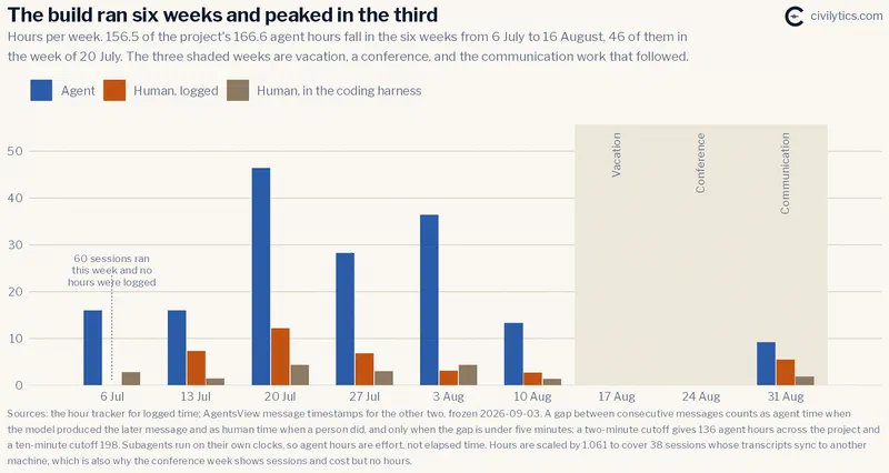
The pattern of the work distribution is pretty clear. After the feasibility assessment of experimenting with this project in April, I was convinced we could do it. With SEAP’s sponsorship, in July I dug in to build the first phase of the dataset focusing just on this century (2000-2023). By the third week the structure was in place and the LLM was able to autonomously stand up the data pipeline — 46 agent hours in that week alone, more than any other. This is where the LLM excelled. But then the leverage — the agent hours I get back for each hour of my own time — slows down as we enter the difficult part of the work: error checking, definition checking, and testing the data, API, and R interfaces to get results and use them ourselves the way someone outside the project would.
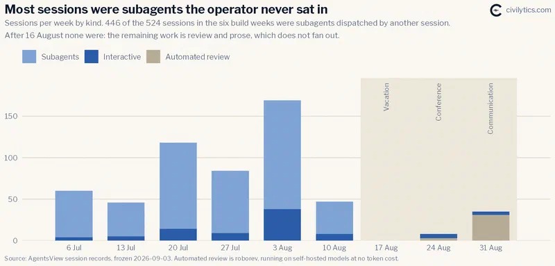
In late July I realized it was feasible to extend the data to the beginning of the time series, 1967, and still meet the contract deadline with SEAP. Moving back in time introduced new data formats and definitional changes, and the work required more interactive sessions with the agent working through the design, reconciling data, and addressing usability questions about the interfaces to the data itself. By this time I was feeling more comfortable using subagents as well, so the overall output really rose.5
How to harness your agent
Just in this short window I rapidly iterated on how I used the LLM to improve the quality of the output per hour. Surrounding the LLM with enabling technologies allows you to work faster and generate higher quality output. Here are four examples:
- Git, and a code forge. 818 commits across the project. Every change is a diff an agent can read, and together the history is a running log to keep continuity across sessions. The R package is public on GitHub (opens in new tab) and installable from r-universe (opens in new tab); the rest currently lives on our own code forge, Gitea (opens in new tab).
- An issue tracker the agent reads and writes. Gitea again. 103 issues closed. This really facilitates project management between me, the human developer, and the LLMs.
- Automated code review. roborev (opens in new tab) uses an LLM to review each change as it lands. I added this to the workflow late and it runs on models hosted on our own hardware, so it costs nothing per token.
- Telemetry. AgentsView (opens in new tab) reads the transcript files each coding tool writes to disk and collects them into one database. I’m storing our agentic work locally to continue to learn how to best use LLMs.
The goal of all this stuff is to enable the LLM and me to collaborate as effectively as possible. One way to think about this is the number of agent hours of output per hour of my input shown in the figure below:
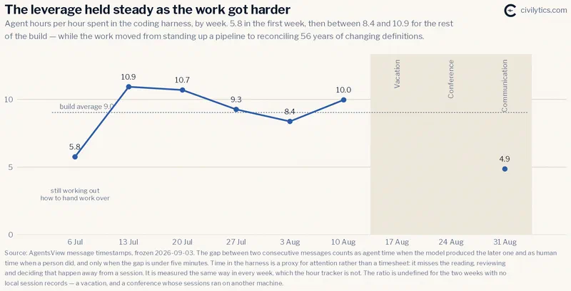
That flat middle is the part I would point at. The work got harder each week, from standing up a pipeline to reconciling definitions across 56 years of collection changes and chasing down esoteric bugs in the pipeline, and the ratio held anyway. I think the machinery above is why: each piece I added and began to use better made the collaboration more effective.
Where the agent hours went
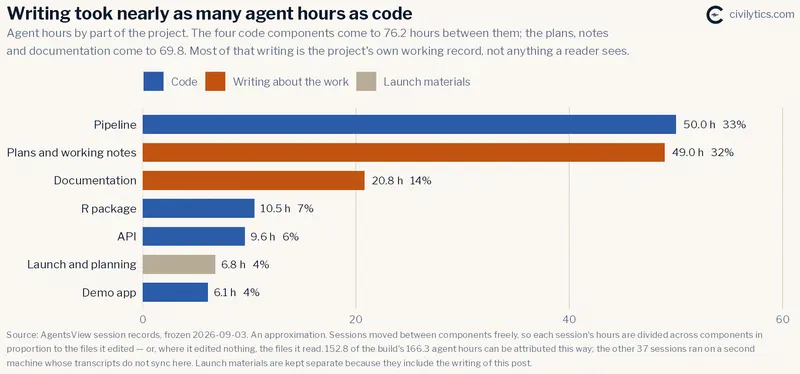
The pipeline is the largest single piece at 50 agent hours, which fits: joining 56 years of Census files is the hard part, and the API, the R package and the demo app are comparatively thin layers over the result. Those three come to 26.2 hours between them. I was really impressed at how quickly, and with little input from me, the LLM was able to add these user-facing layers once we had laid the data and documentation foundation.
Speaking of documentation… a lot of this work is writing and reviewing what to do and giving the LLM clearly structured context to implement. Plans, specifications, progress notes and documentation account for 69.8 agent hours against 76.2 for all four code components combined. Most of that is not documentation anyone outside the project reads. It is the project’s own overhead — a design document before a phase starts, a progress file while it runs, a findings file when it ends. Over the six weeks I got more adept at using this internal project overhead work to scaffold the LLM and set it up for longer running autonomous work.6
How the agents changed
Six weeks is short enough that you would expect to build a thing on one model. But LLM development is fast-paced and even in this window our model mix changed.
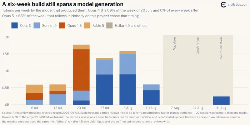
Opus 4.8 wrote 69% of the tokens in the week of 20 July, the heaviest week of the build. It wrote none at all in any week after that. Opus 5 appears at 7% in that same week and is 65% of the next one. The changeover happened in the middle of the hardest stretch of the work, and I did not plan it — a new model came out and I started using it. Most of the Sonnet 5 calls came as subagents created by the Opus sessions — I did not reach for Sonnet models for most of this work. Fable 5 is the other model in the chart: 41% of the first week and a third of the second, then under 8% from the build’s peak week onward.
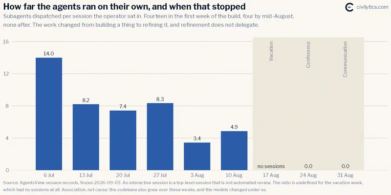
In the first week of July, every session I sat in handed fourteen pieces of work to subagents — the shape you use when the task is large and its parts are not yet known. By early August that is down to three or four, and the first week of August is 38 interactive sessions instead of nine: the work had become a long list of specific things to fix rather than a few things to figure out.
What this means for a small firm
A six week build period of fairly intense LLM use has allowed us to make something production grade and ready for others to use. This class of public-good data infrastructure was previously not economically possible for us to produce as a two-person firm, and now it is — if the two people know the domain well and work thoughtfully with this new class of tools.
We brought our expertise and familiarity with the data, earned through many years of doing analyses for community organizations across the country. We also brought a social scientist’s habit to the question of how to work with an LLM: treat the process as something to measure, instrument it, and check whether it did what you thought it did. This post is an example of that!
One thing we have not yet measured is how often the model was wrong and how those mistakes were caught and fixed. That is the number this post cannot give you. We’ll dive into LLM chat transcripts in a subsequent post to analyze the interplay between our subject matter expertise and the LLMs’ coding expertise.
Appendix: Where the tokens went
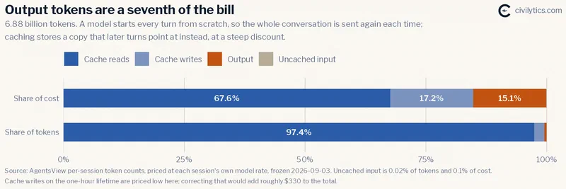
For readers already building with agents, here is where the 6.88 billion tokens went.
| Token class | Tokens | Share of cost |
|---|---|---|
| Cache reads | 6,701,638,627 | 67.6% |
| Cache writes | 145,969,913 | 17.2% |
| Output | 31,315,836 | 15.1% |
| Uncached input | 1,194,773 | 0.1% |
Output tokens are the number everyone reaches for, and they are a seventh of the bill. A model starts every turn from scratch, so the whole conversation is sent again each time. Caching stores a copy that later turns can point at instead of resending it, at a steep discount — and at 6.7 billion cache-read tokens the discount stops mattering. Two-thirds of what this project cost was re-reading context the model had already been given.7
62 of these hours were logged in our time tracker and attributed to our sponsor for billing purposes. I’m estimating the remaining hours because this was a passion project and I didn’t always track those hours. That tracking was particularly light at the beginning, during the feasibility phase, and at the end, like right now when I’m working on the communication materials. ↩︎
97.5% of cities under 50,000 people reported in FY2022 which was the last published census year. You’ll see us quote 2022 numbers frequently as a result. ↩︎
April was 21.5 logged hours and 153 commits, spent finding out whether a language model could do this work at all. It has no session record — Claude Code deleted its transcripts after 30 days by default, and we raised that setting a month too late. Raise your transcript retention before you need it. ↩︎
List-price equivalent, not money spent. 492 of the 569 sessions ran on a subscription, and the figure is computed by multiplying token counts against a published price list rather than read off an invoice. April is not in it; pricing that month off July, the nearest comparable one, puts the whole project between $5,500 and $5,800 in token costs at the market rate. ↩︎
Subagents run at the same time as each other and as the session that started them, so several agents can be working through the same hour and each one is counted. Read agent hours as effort, not elapsed time — 166.6 hours of effort is 147.0 hours in which any agent was running at all. Weekly and monthly groupings assign an idle gap to different periods, so the table above sums to 165.7 for July to September against 166.6 for the project. ↩︎
The split is an approximation. Sessions moved between the components freely, so each session’s hours are divided in proportion to the files it touched rather than assigned to one of them. The launch materials are counted on their own line, since they include the writing of this post. ↩︎
One known understatement. 45% of the cache writes used the one-hour cache lifetime, which lists at twice the base input rate rather than the 1.25× used in the price table behind these figures. If that is right, the list-price equivalent is about $330 higher than the total above. ↩︎